1: Viewing a grid in the Short Drinks sample
The Short Drinks sample consists of an .
mdd file (
short_drinks.mdd) and case data in the form of a SQL Server backup of a relational MR (RDB) database. Before you can do the exercises in this topic, you need to restore the backup. To do this you need to have SQL Server Client Tools installed. For more information, see
Restoring the Short Drinks sample database.
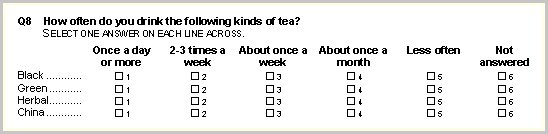
The Short Drinks survey contains several grid questions. A grid question can be considered a loop in which the iterations are controlled by a category list and therefore the maximum number of iterations is known. Look in particular at the frequenz grid, which is based on a question that asks respondents to say how often they drink various types of tea:
The frequenz grid is the last question in the questionnaire. In the metadata, this grid is made up of a Grid object called frequenz. The iterations of the grid are controlled by a category list that contains categories for the different types of tea. Nested inside the Grid object is a single categorical question called questi2 that contains the frequency categories.
The OLE DB implementation of the Relational MR Database CDSC (RDB DSC 2) presents the case data in the flat VDATA virtual table and hierarchical HDATA virtual tables.
First, open DM Query.
1 In Windows Explorer, go to the folder in which DM Query was installed. By default, this is [INSTALL_FOLDER]\IBM\SPSS\DataCollection\7\DDL\Code\Tools\VB6\DM Query. Then double-click the DM Query.exe file.
Now connect to the Short Drinks database using RDB DSC 2.
2 From the DM Query File menu, choose New Connection.
This opens the Connection tab in the Data Link Properties dialog box.
3 From the Metadata Type list, select Intelligence Metadata Document.
4 Enter the Metadata Location: Click Browse, navigate to the folder in which the Short Drinks sample .mdd file was installed, and then select it. By default, it is installed in:
[INSTALL_FOLDER]\IBM\SPSS\DataCollection\7\DDL\Data\Mdd
5 From the Case Data Type list, select Intelligence Database (MS SQL Server) (read-write).
6 In
Case Data Location, type the OLE DB connection string. Typically the default OLE DB connection string stored in the .
mdd file is displayed, but you may need to change the server name to reflect the name of the server on which you restored the database. For more information, see
Connecting to a relational MR database using RDB DSC 2.
7 Enter short_drinks in the Case Data Project text box.
8 Click the Advanced tab, and from the Categorical Variables list, select Return data as category names.
9 Click OK.
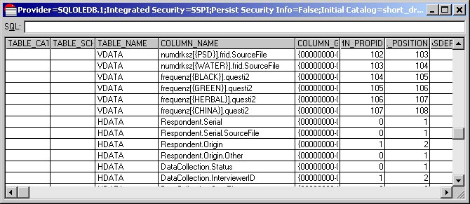
10 Look at the schema. You do this by choosing Columns from the Schema menu in DM Query.
The TABLE_NAME and COLUMN_NAME columns show the names of the tables and columns in the virtual table schema. Use the scroll bar to scroll down the list. The columns in the VDATA virtual table are listed first. The last four VDATA columns are the columns that store the responses to the frequenz grid in a flattened form:
frequenz[{BLACK}].questi2
frequenz[{GREEN}].questi2
frequenz[{HERBAL}].questi2
frequenz[{CHINA}].questi2
Because VDATA is a flat table, any hierarchical data must be flattened before it can be represented in the table. This means that one column is used to store the responses to each question each time it is asked (that is, in each iteration). The frequenz grid contains only one question (questi2) and the iterations correspond to the rows of the grid question as it is displayed above. Therefore there is one column for each row of the grid question.
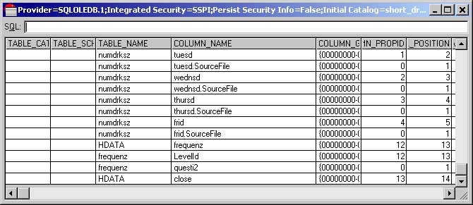
11 Scroll to see the names of the columns in the HDATA top-level hierarchical table. These columns store the responses to simple questions that are not nested inside a loop or grid. Further down are tables called childhz, numdrkz, and frequenz. These are second-level tables that store the responses to the three grid questions.
The frequenz table contains two columns: LevelId and questi2. The LevelId column stores the name of the category that drives the iteration and the questi2 column stores the response for that iteration. (The numdrnkz table contains more columns because there are several numeric questions nested inside the numdrnkz grid, and each of these numeric questions has an associated source file helper variable.)
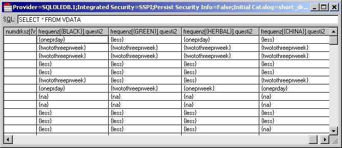
12 Run a query on the flat VDATA table by entering the following into the text box and pressing Enter:
SELECT * FROM VDATA
This query selects all of the columns in the VDATA virtual table. If you scroll through the columns, you will eventually see the four columns that store the responses to the frequenz grid in a flattened form:
Each of these columns stores the response chosen for a single row of the grid question.
13 Run a query on the HDATA hierarchical tables by entering the following into the text box and pressing Enter:
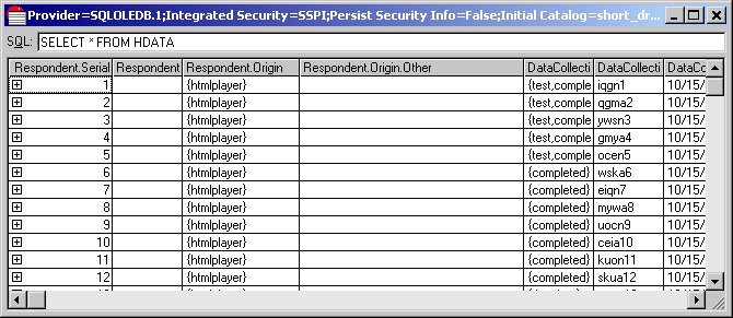
SELECT * FROM HDATA
When you are looking at the results of an HDATA query in DM Query, you can expand and collapse all of the rows or individual rows. Click the + and - symbols in the top left corner of the first column to expand and collapse an individual row. Select Expand all rows and Collapse all rows from the View menu to expand and collapse all of the rows.
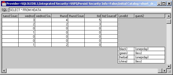
14 Expand the first row and scroll to the right. First are the HDATA columns that store the responses to the simple questions that are not nested in a loop or grid. Next are the three tables that store the responses to the three grids in a hierarchical form. Scroll to the end to see the frequenz table that stores the responses to the frequenz grid question.
The responses are identical to the responses shown for the first respondent in the columns returned from the flat VDATA table, but this time the responses are stored in one column with the response for each iteration stored in a separate row. The LevelID column stores the name of the category that controls the iteration.
This demonstrates that RDB DSC 2 provides two views of the data: one in the flat VDATA virtual table and one in the hierarchical HDATA virtual tables. Both views are available automatically when you connect using an MDM Document. If you connect without an MDM Document, the HDATA view is not available.
Why use the hierarchical view?
You may be wondering what is the advantage of having the additional hierarchical view of the data. Why not just use with the flat VDATA view? The answer is that there are several advantages to the hierarchical view:
▪It is more efficient to store the data collected with loops and grids hierarchically, particularly when each respondent is asked only some of the iterations, because storage space is not wasted for the iterations that are not asked.
▪It is the only way of representing unbounded loops (these are loops for which the maximum number of iterations is undefined), because flattening the data requires knowing the total number of iterations.
▪It easier to perform calculations on hierarchical data. For example, here is the query that you need to use to return the responses to a grid question (and the serial number variable) from the flat VDATA table:
SELECT Respondent.Serial, frequenz[{BLACK}].questi2,
frequenz[{GREEN}].questi2, frequenz[{HERBAL}].questi2,
frequenz[{CHINA}].questi2
FROM VDATA
The equivalent query against HDATA is much simpler:
SELECT Respondent.Serial, frequenz FROM HDATA
▪Similarly, it is easier to perform aggregation of hierarchical data using the hierarchical view. For example, here is a query that returns a count of the responses to a grid question (and the serial number variable) from the flat VDATA table:
SELECT Respondent.Serial, Iif(frequenz[{BLACK}].questi2 IS Null, 0, 1) +
Iif(frequenz[{GREEN}].questi2 IS Null, 0, 1) +
Iif(frequenz[{BLACK}].questi2 IS Null, 0, 1) +
Iif(frequenz[{HERBAL}].questi2 IS Null, 0, 1)
FROM VDATA
The equivalent query against HDATA is much simpler:
SELECT Respondent.Serial, frequenz.(COUNT(questi2)) FROM hdata
For more information, see
Hierarchical SQL queries.
Like RDB DSC 2, Quanvert DSC also provides both views of the data. The next section explains more about unbounded loops.
See also