Understanding population levels
Sample script file: HierarchicalData.mrs
This example script is based on the Household sample data set. See
Running the sample table scripts for information on running the example scripts.
When you use the hierarchical view of the data, you need to understand the significance of populating tables at the various hierarchical levels. To illustrate this we will use the Household sample data. (See
The Household sample.) It represents the data collected using the following fictitious survey:
▪Household questions. Respondents are asked a number of questions about their household as a whole, such as address, age of the building, and number of rooms.
▪Person questions. Respondents are then asked a number of questions about each person in the household, such as the person's name, age, gender, and occupation, and a grid question that asks the number of days he or she watches various TV channels.
▪Overseas trip questions. Each person is also asked a number of questions about each overseas trip that he or she has taken in the previous year (if any), such as the purpose of the trip, number of days he or she was away from home, and countries that were visited.
▪Vehicle questions. Finally, respondents are asked a number of questions about each vehicle that belongs to their household (if any), such as the vehicle's type, color, and annual mileage, and a grid question that asks the respondent to rate the vehicle's features.
Loops called person, trip, and vehicle are used to ask the person, overseas trip, and vehicle questions, respectively. The loops are iterated (and therefore the questions are asked) as many times as necessary. For example, in a household of three people, the person loop will be iterated three times, whereas in a single-person household it will be iterated once. In a household that has no cars, bikes, or other vehicles, the vehicle questions will not be asked at all and the vehicle loop will have no iterations.
In the Quanvert database, each of the loops corresponds to an Array object of type mlLevel in the metadata and a child table (called a level) in the case data. (In the XML data set, the person Array object is of type mlExpand.) Each record in a child table is considered a case at that level and corresponds to one iteration of its corresponding loop. This means that the three-person household will have three records in the person child table and this corresponds to three person-level cases.
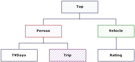
The structure of the levels corresponds to the structure of the loops. This means that because the trip loop is nested within the person loop, the trip level is a child of the person level. The two grids are also represented in the case data as levels, each nested within its parent level. The following diagram shows the levels structure.
Figure 1. Structure of levels
When you are using a hierarchical view of the data, you can define the level at which each table is to be populated. The level that you choose affects the figures that are shown in the cells of the table. When you populate a table at the top (HDATA) level, each case corresponds to a household and therefore the counts show numbers of households; when you populate the table at the person level, each case corresponds to a person and therefore the counts show numbers of people; when you populate a table at the trip level, each case is an overseas trip and the counts show numbers of trips, etc. To illustrate this, let's look at some tables.
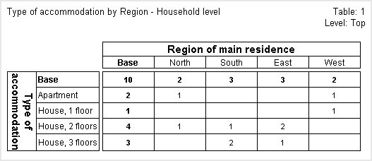
Table 1: Top-level variables tabulated at the top level
This table crosstabulates two top-level variables (housetype and region) and is populated at the top (HDATA) level. The counts in the cells refer to households because in this survey the top-level questions refer to households. Notice that the cell in the top left corner of the table shows that there are 10 households in the sample.
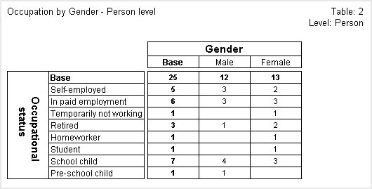
Table 2: Person-level variables tabulated at the person level
This table crosstabulates two person-level variables (occupation and gender) and is populated at the person level. Each cell shows the number of people of a given occupation and gender. Looking at the top left cell, we can see that there are 25 cases at the person level, or, to put it another way, there are 25 people in the sample.
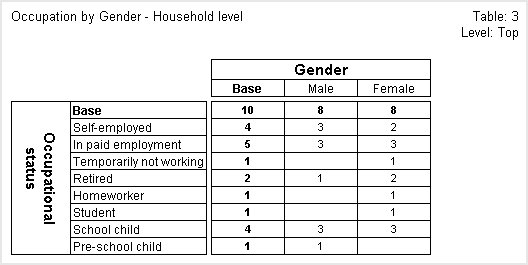
Table 3: Person-level variables tabulated at the top level
This table crosstabulates the same two person-level variables, but this time the table is populated at the top (HDATA) level. This means that instead of showing the number of people of a given occupation and gender, each cell now shows the number of households that contain people of the given occupation and gender. The top left cell shows that the base for the table is the same as in
Table 1: Top-level variables tabulated at the top level. This is what you would expect because both tables are counting the number of households and are unfiltered, and every household contains at least one person.
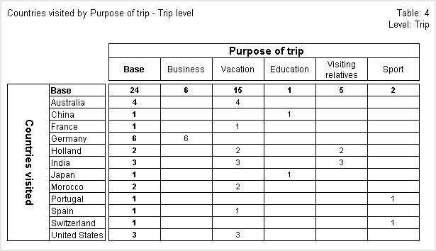
Table 4: Trip-level variables tabulated at the trip level
The following table crosstabulates two trip-level variables (country and purpose) and is populated at the trip level. This means that each cell shows the number of overseas trips that involved a particular country and purpose. Looking at the top left cell, we can see that there were a total of 24 overseas trips (or to put it another way, there are 24 cases at the trip level).
Table 5: Trip-level variables tabulated at the person level
The following table crosstabulates the same two trip-level variables, but this time the table is populated at the person level. This means that instead of showing the number of overseas trips that involved a particular country and purpose, each cell now shows the number of people that took trips that involved a particular country and purpose. Looking at the top left cell, we can see that the base for the table is 12. This is less than the base in
Table 2: Person-level variables tabulated at the person level (which tabulates two person-level variables at the person level) because some people did not take an overseas trip and therefore there are no records (cases) at the trip level for those people.
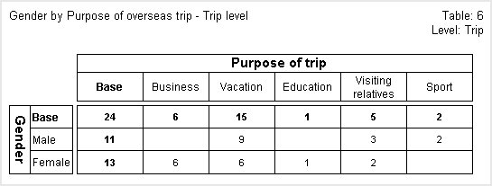
Table 6: Variables from different levels tabulated at the default level
You can create tables that use variables from more than one level. The following table crosstabulates a person-level variable (gender) with a trip-level variable (purpose). When you use variables from parent and child levels like this, the population level defaults to the level of the lowest-level variable, which is the trip level in this example. This means that each cell in this table shows the number of overseas trips for a particular purpose and the gender of the person who took them. If we look at the Base column, we can see that of the 24 overseas trips that were taken, 11 were taken by males and 13 by females.
The base for the table (24) is the same as the base in
Table 4: Trip-level variables tabulated at the trip level (which tabulates two trip-level variables at the trip level).
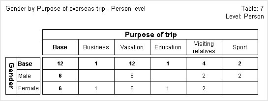
Table 7: Variables from different levels tabulated at a higher level
The following table crosstabulates the same person-level variable (gender) with the same trip-level variable (purpose). However, this time the table is populated at the person level. This means that instead of showing the number of overseas trips, each cell now shows the number of people of each gender who took trips that involved a particular purpose. If we look at the Base column, we can see that of the 12 people who took overseas trips, 6 were males and 6 were females.
The top left cell shows that the base for the table is 12, which corresponds with the base in
Table 5: Trip-level variables tabulated at the person level, which tabulates two trip-level variables at the person level. The base counts every person who took one or more overseas trips. People who did not take an overseas trip are not counted in the base because the base calculation considers empty levels to be Null.
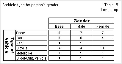
Table 8: Tabulating variables from different “parallel” levels
The following table crosstabulates a variable from the vehicle level (vehicletype) with a person-level variable (gender). If you scroll back to the diagram that shows the levels structure, you will see that the person and vehicle levels are parallel to each other (on different branches of the tree). This means that the data at the two levels is not directly related to each other. It would therefore make no sense to populate the table at either the person or vehicle level and therefore this is not allowed. However, you can populate the table at a higher level that is an ancestor of both of them. In this example, the only level that is an ancestor of both the person and vehicle levels is the top (HDATA) level. Each cell therefore shows the number of households that have the various types of vehicles and that contain people of the given gender.
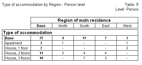
Table 9: Tabulating variables from higher levels at a lower level
You can also tabulate higher level variables at a lower level, provided that the variables are on the same branch of the structure and are not on parallel branches. The following table crosstabulates two top-level variables (housetype and region) as for table 1, but this time is populated at the person level. The counts in the cells refer to people rather than households. The cell in the top left corner of the table shows that there are 25 people in the sample.
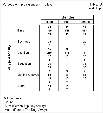
Table 10: Showing summary statistics of a numeric variable in the cell contents
In this table, the cell contents show not only the counts, but also the sum and mean summary statistics of the DaysAway numeric variable. This is a trip-level variable that stores the length of the trip in days. The sum values show the total number of days away and because the table is populated at the trip level, the mean values show the mean number of days per trip.
In the top left cell of the table, the first figure is 24, which corresponds with the base in
Table 4: Trip-level variables tabulated at the trip level, which tabulates two trip-level variables at the trip level. This figure shows the total number of overseas trips that were taken. The next figure is 320, which is the total number of days for all the trips. The final figure is the mean, which shows the average number of days per trip.
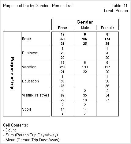
If you now populate the table at the person level, the sum values stay the same, but the mean values show the average number of days per person instead of per trip. Here is the table populated at the person level.
Look at the three figures in the top left cell of this new table. The first figure is 12, which corresponds with the base in
Table 7: Variables from different levels tabulated at a higher level, which tabulates the same variables at the person level. This figure shows the total number of people who have taken at least one overseas trip. The next figure is 320, which is the total number of days for all the trips. This figure is the same as when we populated the table at the trip level. However, the mean value is now 27, because it now shows the average number of days away per person instead of per trip.
Using weighting variables with hierarchical data
When you use weighting variables, the level of the weighting variable restricts the levels at which you can populate the table. See Weighting for more information.
See also
